Variant Calling and Ancestry Inference
Assignment Overview
Modern genome sequencing technologies produce sequencing “reads” which represent subsequences of the fragmented DNA molecules isolated in an experiment. Last week, you practiced aligning (or “mapping”) reads to a reference genome, visualizing and summarizing the contents of the resulting alignment files.
For many DNA-based applications, a next step would be to identify sites where samples vary from the reference. By comparing patterns of variation at in a sample of genomes, we can infer ancestry relationships, as well as genomic locations of historical recombination events (i.e., genome shuffling during meiosis).
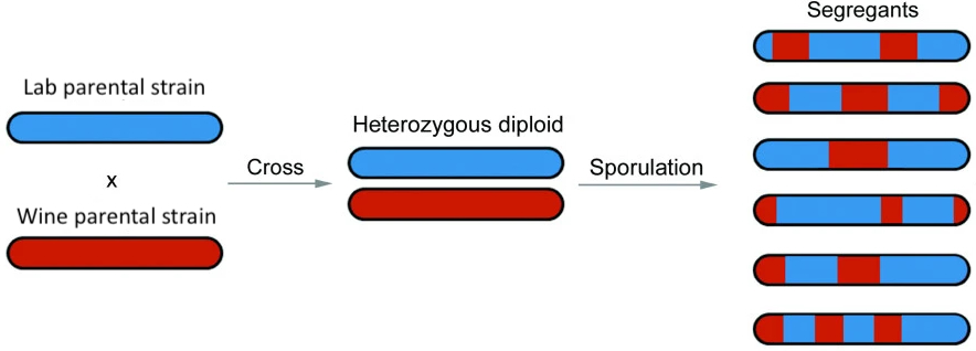
As with part of last week’s lab, you will work with Illumina short-read sequencing data from a cross between a lab strain of Saccharomyces cerevisiae and a wine strain, as described in the paper: “Finding the sources of missing heritability in a yeast cross”. Diploid offspring from this cross were sporulated, and a colony from one haploid spore from each tetrad was sequenced. Thus, the data represent segregants, which are haploid whose genomes resemble a mosaic of the two parental strains.
We have preprocessed the sequencing reads and aligned them to the yeast reference genome (sacCer3). You will begin at the stage of variant discovery and exploratory analysis, then move to ancestry inference, and finally implement a simple method to detect meiotic crossovers.
Exercise 1: Data preprocessing and variant calling
Place all of your code for Exercise 1 in a bash script called call_variants.sh.
You will be provided with pre-aligned sequencing reads for 10 yeast segregants (BAM files):
Make sure your .gitignore excludes this file and the BAM files it contains; you should not upload them with your assignment.
Download the file and extract it with:
tar -xzvf BYxRM_bam.tar.gz
You should now see a directory containing 10 bam files. Navigate into this directory for the following steps.
Step 1.1: Index each of your bam files with samtools index. You should now see 10 files with the suffix .bam.bai.
Question 1.1: How many aligned reads does each BAM file contain? (Hint: See the -c flag for samtools view). Store these counts in a new file called read_counts.txt. Storing the file names alongside the counts is optional.
Step 1.2: Generate a list of bam file names (one bam file per line) and name it bamListFile.txt. Its first lines look like this:
A01_09.bam
A01_11.bam
A01_23.bam
...
We are now ready to discover variants–differences between the reference genome and each of your aligned haploid samples–using a program called FreeBayes. Some of these commands are a bit esoteric, so I have provided the most of the steps below, but please fill in the missing pieces (indicated with blank lines _________).
As these commands take a long time to run, feel free to get them going in a separate window, but I will provide you with the output file here so that you can move on to the next exercise in the meantime: biallelic.vcf
# run FreeBayes to discover variants
freebayes -f _________ -L _________ --genotype-qualities -p _________ > unfiltered.vcf

# the resulting VCF file is unfiltered, meaning that it contains low-confidence calls and also has some quirky formatting, so the following steps use a software suite called vcflib to clean up the VCF

# filter the variants based on their quality score and remove sites where any sample had missing data
vcffilter -f "QUAL > 20" -f "AN > 9" unfiltered.vcf > filtered.vcf

# FreeBayes has a quirk where it sometimes records haplotypes rather than individual variants; we want to override this behavior
vcfallelicprimitives -kg filtered.vcf > decomposed.vcf

# in very rare cases, a single site may have more than two alleles detected in your sample; while these cases may be interesting, they may also reflect technical errors and also pose a challenge for parsing the data, so we remove them
vcfbreakmulti decomposed.vcf > biallelic.vcf
Exercise 2: Exploratory Data Analysis
Now that you have discovered and genotyped variants in your samples, you would like to do some basic exploratory analysis of the patterns you observe in the VCF.
You will be creating figures that explore the following features of the data:
- The allele frequency spectrum of the discovered variants
- The distribution of read depth across sample genotypes
Create an empty ex2.py script now where you’ll be doing the analyses in the next steps.
Step 2.1: Parse the VCF file
For these analyses, you’ll have to parse the VCF file that we provided. If you can find a python library that handles VCF parsing, you’re welcome to use it, but it may be easier to simply use the following structure:
for line in open(<vcf_file_name>):
    if line.startswith('#'):
        continue
    fields = line.rstrip('\n').split('\t')

    # grab what you need from `fields`
Each of the following analyses needs information from a different field/column from the VCF. As such, you’ll be grabbing multiple pieces of information from each line, so if you do use this structure, instead of looping through the VCF separately for each analysis, try to use just a single loop across all analyses.
Remember, you can read more about the VCF file format here.
Step 2.2: Allele frequency spectrum
Using your Python script above, extract the allele frequency of each variant and output it to a new file called AF.txt which contains only the allele frequencies – one per line (potentially having the first line contain a header). This information is pre-calculated for you and can be found in the variant specific INFO field. Check the file header to decide which ID is appropriate. This is a per-variant metric, so with 20 variants and 10 samples, you would only have 20 allele frequencies.
Use R to plot a histogram showing the allele frequency spectrum (distribution) of the variants in the VCF.
Make sure you label the panel appropriately. Set bins=11 to avoid binning artifacts.
Question 2.1: Interpret this figure in two or three sentences in your own words. Does it look as expected? Why or why not? Bonus: what is the name of this distribution?
Step 2.3: Read depth distribution
Using your Python script above, extract the read depth of each variant site in each sample and output it to a new file called DP.txt which contains only the depths – one per line (potentially having the first line contain a header). This information can be found in the sample specific FORMAT fields and the end of each line. Check the file header to decide which ID is appropriate. This is a per-sample, per-variant metric, so with 20 variants and 10 samples, you would have 200 read depths.
Plot a histogram showing the distribution of read depth at each variant across all samples (i.e., a single histogram, rather than multiple histograms stratified by sites or samples).
Make sure you label the plot appropriately. Set bins=21 and xlim(0, 20) to make the figure more legible, noting that some very high depths will be cut off.
Question 2.2: Interpret this figure in two or three sentences in your own words. What does it represent? Does it look as expected? Why or why not? Bonus: what is the name of this distribution?
Exercise 3: Ancestry Inference
Consider the experimental design and examine the figure posted in the Assignment Overview section. Note that the reference genome sacCer3 is itself derived from the lab strain. The implication is that regions of the segregant genomes that derive from the lab strain should be largely carry alleles that match the reference genome, whereas regions of the segregant genome that derive from the wine strain should be enriched for differences (alternative alleles) compared to the reference genome.
Step 3.1: Visualize data in IGV
Load all 10 sample BAM files into IGV simultaneously. Set the browser to chrIV:192829-205454.
Question 3.1: Which samples do you think derive from the lab strain and which samples do you think derive from the wine strain in this region of the genome?
Step 3.2: Infer sample ancestry
Write a Python script that parses a VCF and converts it to “long” format. Each line of the output file (which you can call gt_long.txt) should contain:
- the sample ID
- the chromosome of the variant
- the position of the variant
- the genotype of your sample (reference
0or alternative1)
Here is some pseudocode to get you started:
# sample IDs (in order, corresponding to the VCF sample columns)
sample_ids = ["A01_62", "A01_39", "A01_63", "A01_35", "A01_31",
              "A01_27", "A01_24", "A01_23", "A01_11", "A01_09"]

# open the VCF file
for each line in the VCF file:
    if line starts with "#":
        skip it, as these are metadata

    # split the line into fields by tab, then
    chrom = fields[0]
    pos   = fields[1]

    # for each sample in sample_ids:
        # get the sample's data from fields[9], fields[10], ...
        # genotypes are represented by the first value before ":" in that sample's data
        # if genotype is "0" then print "0"
        # if genotype is "1" then print "1"
        # otherwise skip
Step 3.3: Visualize the ancestry of one sample and one chromosome
For a chromosome chrII of sample A01_62, create a figure where the x axis is the position and colors indicate whether the genotype was a 0 or a 1. Make sure to convert the genotype to a factor variable.
Question 3.2: Do you notice any patterns? What do the transitions indicate?
Step 3.4: Expand your visualization
Now use facet_grid to plot all chromosomes for sample A01_62. Use the scales = "free_x" and space = "free_x" options to allow for different x-axis scales for different chromosomes. Extend your plot to consider all samples. Note that different samples do not need their own facets, but can simply be arranged along the y axis (which can accept variables that are not numeric!).
Exercise 4 (Optional extension): Detecting meiotic crossovers
One of the most important aspects of meiosis is crossover recombination. In these yeast segregants, each haploid genome contains multiple crossover events, visible as switches from long tracts of BY ancestry to long tracts of RM ancestry (or vice versa).
Step 4.1: Write code to detect crossovers
Extend your ancestry inference script to detect sites of ancestry switches.
Question 4.1: Do you think a single “discordant” SNP is sufficient to call a crossover? Why or why not?
Adjust your code accordingly to attempt to discover true crossovers.
- Count the number of crossover events per sample.
- Record these counts into a text file (e.g.,
crossovers.txt).
Step 4.2: Make a histogram
In R, create a histogram showing the number of crossovers per segregant across the 10 samples. Save as crossovers.png.
Question 4.2: What does the distribution of crossovers look like? How does it compare to expectations for yeast meiosis (literature values ~50–90 cM per meiosis, corresponding to several crossovers per chromosome)?
Submission
- Bash script to produce the VCF file in Exercise 1 (
ex1.sh) - Python script to produce the input necessary for plots in Exercise 2 (
ex2.py) - R script to generate figures for Exercise 1 (with answers to written questions as comments;
ex2.R) - Python script to perform ancestry inference in Exercise 3 (
ex3.py) - R script to generate ancestry figures in Exercise 3 (
ex3.R) - Optional: Python script to detect crossovers in Exercise 4 (
ex4.py) - Optional: R script to generate the crossover histogram (
ex4.R) - Figures as PNGs